Introduction
fredr provides a complete set of R bindings to the Federal Reserve of Economic Data (FRED) RESTful API, provided by the Federal Reserve Bank of St. Louis. The functions allow the user to search for and fetch time series observations as well as associated metadata within the FRED database.
The core function in this package is fredr(), which fetches observations for a FRED series. That said, there are many other FRED endpoints exposed through fredr, such as fredr_series_search_text(), which allows you to search for a FRED series by text.
We strongly encourage referencing the FRED API documentation to leverage the full power of fredr.
Authentication
To use fredr and the FRED API in general, you must first obtain a FRED API key. It is also recommended to review the FRED API Terms of Use.
Once you’ve obtained an API key, the recommended way to use it is to set the key as an environment variable: FRED_API_KEY . The easiest way to do that is by calling usethis::edit_r_environ() to open a .Renviron file. Once the file is open set the key as:
FRED_API_KEY=abcdefghijklmnopqrstuvwxyz123456where the key has been replaced by the one you received from FRED. Don’t forget to restart R after saving and closing the .Renviron file.
Alternatively, you can set an API key for the current R session with fredr_set_key() like so:
fredr_set_key("abcdefghijklmnopqrstuvwxyz123456")Again, this will only set the key for the current R session, and it is recommended to use an environment variable.
Retrieve series observations
fredr() (an alias for fredr_series_observations()) retrieves series observations (i.e. the actual time series data) for a specified FRED series ID. The function returns a tibble with 3 columns (observation date, series ID, and value).
fredr(
  series_id = "UNRATE",
  observation_start = as.Date("1990-01-01"),
  observation_end = as.Date("2000-01-01")
)
#> # A tibble: 121 × 5
#>    date       series_id value realtime_start realtime_end
#>    <date>     <chr>     <dbl> <date>         <date>
#>  1 1990-01-01 UNRATE      5.4 2023-04-17     2023-04-17
#>  2 1990-02-01 UNRATE      5.3 2023-04-17     2023-04-17
#>  3 1990-03-01 UNRATE      5.2 2023-04-17     2023-04-17
#>  4 1990-04-01 UNRATE      5.4 2023-04-17     2023-04-17
#>  5 1990-05-01 UNRATE      5.4 2023-04-17     2023-04-17
#>  6 1990-06-01 UNRATE      5.2 2023-04-17     2023-04-17
#>  7 1990-07-01 UNRATE      5.5 2023-04-17     2023-04-17
#>  8 1990-08-01 UNRATE      5.7 2023-04-17     2023-04-17
#>  9 1990-09-01 UNRATE      5.9 2023-04-17     2023-04-17
#> 10 1990-10-01 UNRATE      5.9 2023-04-17     2023-04-17
#> # ℹ 111 more rows
Leverage the native features of the FRED API by passing additional parameters:
fredr(
  series_id = "UNRATE",
  observation_start = as.Date("1990-01-01"),
  observation_end = as.Date("2000-01-01"),
  frequency = "q", # quarterly
  units = "chg" # change over previous value
)
#> # A tibble: 41 × 5
#>    date       series_id   value realtime_start realtime_end
#>    <date>     <chr>       <dbl> <date>         <date>
#>  1 1990-01-01 UNRATE    -0.0667 2023-04-17     2023-04-17
#>  2 1990-04-01 UNRATE     0.0333 2023-04-17     2023-04-17
#>  3 1990-07-01 UNRATE     0.367  2023-04-17     2023-04-17
#>  4 1990-10-01 UNRATE     0.433  2023-04-17     2023-04-17
#>  5 1991-01-01 UNRATE     0.467  2023-04-17     2023-04-17
#>  6 1991-04-01 UNRATE     0.233  2023-04-17     2023-04-17
#>  7 1991-07-01 UNRATE     0.0333 2023-04-17     2023-04-17
#>  8 1991-10-01 UNRATE     0.233  2023-04-17     2023-04-17
#>  9 1992-01-01 UNRATE     0.267  2023-04-17     2023-04-17
#> 10 1992-04-01 UNRATE     0.233  2023-04-17     2023-04-17
#> # ℹ 31 more rows
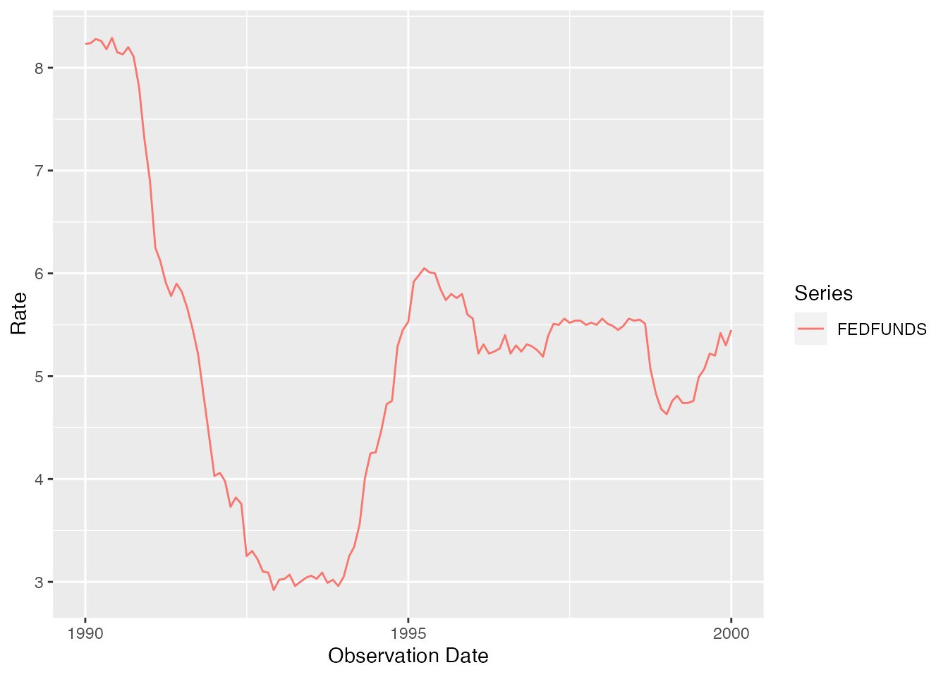
fredr plays nicely with tidyverse packages:
library(dplyr)
library(ggplot2)

popular_funds_series <- fredr_series_search_text(
    search_text = "federal funds",
    order_by = "popularity",
    sort_order = "desc",
    limit = 1
)

popular_funds_series_id <- popular_funds_series$id

popular_funds_series_id %>%
  fredr(
    observation_start = as.Date("1990-01-01"),
    observation_end = as.Date("2000-01-01")
  ) %>%
  ggplot(data = ., mapping = aes(x = date, y = value, color = series_id)) +
    geom_line() +
    labs(x = "Observation Date", y = "Rate", color = "Series")
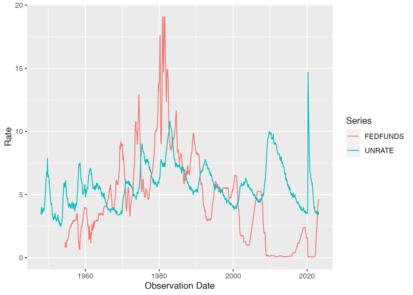
Since fredr() returns a tibble with a series ID, mapping fredr() over a vector of series IDs can be achieved as follows:
library(purrr)

map_dfr(c("UNRATE", "FEDFUNDS"), fredr) %>%
  ggplot(data = ., mapping = aes(x = date, y = value, color = series_id)) +
    geom_line() +
    labs(x = "Observation Date", y = "Rate", color = "Series")
Using purrr::pmap_dfr() allows you to use varying optional parameters as well.
params <- list(
  series_id = c("UNRATE", "OILPRICE"),
  frequency = c("m", "q")
)

pmap_dfr(
  .l = params,
  .f = ~ fredr(series_id = .x, frequency = .y)
)
#> # A tibble: 1,174 × 5
#>    date       series_id value realtime_start realtime_end
#>    <date>     <chr>     <dbl> <date>         <date>
#>  1 1948-01-01 UNRATE      3.4 2023-04-17     2023-04-17
#>  2 1948-02-01 UNRATE      3.8 2023-04-17     2023-04-17
#>  3 1948-03-01 UNRATE      4   2023-04-17     2023-04-17
#>  4 1948-04-01 UNRATE      3.9 2023-04-17     2023-04-17
#>  5 1948-05-01 UNRATE      3.5 2023-04-17     2023-04-17
#>  6 1948-06-01 UNRATE      3.6 2023-04-17     2023-04-17
#>  7 1948-07-01 UNRATE      3.6 2023-04-17     2023-04-17
#>  8 1948-08-01 UNRATE      3.9 2023-04-17     2023-04-17
#>  9 1948-09-01 UNRATE      3.8 2023-04-17     2023-04-17
#> 10 1948-10-01 UNRATE      3.7 2023-04-17     2023-04-17
#> # ℹ 1,164 more rows
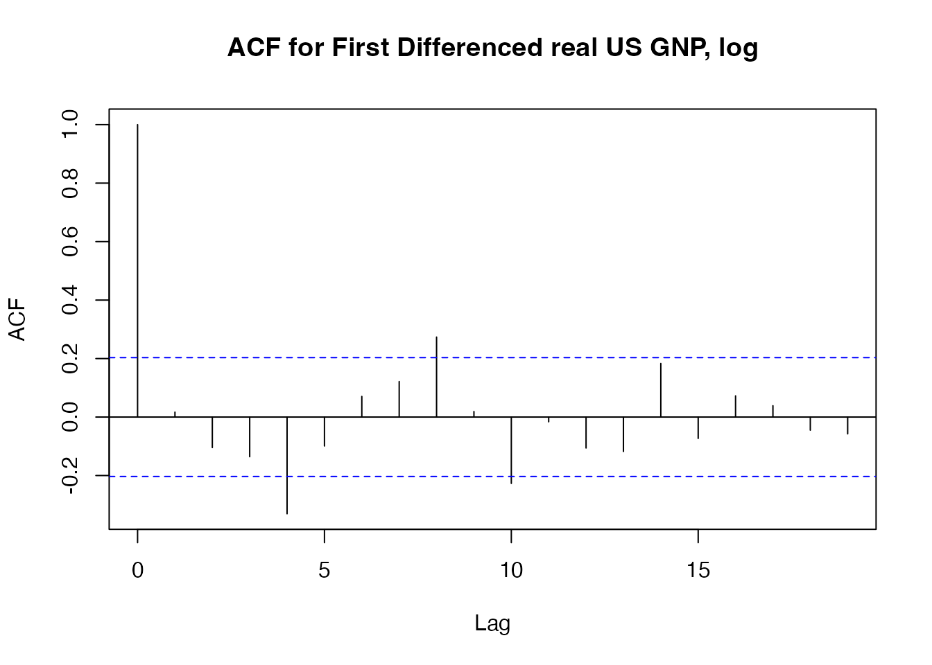
It is relatively straightforward to convert tibbles returned by fredr into other time series objects. For example:
library(xts)

gnpca <- fredr(series_id = "GNPCA", units = "log") %>%
  mutate(value = value - lag(value)) %>%
  filter(!is.na(value))

gnpca_xts <- xts(
  x = gnpca$value,
  order.by = gnpca$date
)

gnpca_xts %>%
  StructTS() %>%
  residuals() %>%
  acf(., main = "ACF for First Differenced real US GNP, log")
Endpoints
fredr implements functions for all FRED API endpoints. For usage examples for these functions, please consult the relevant vignette:
Finally, fredr is packaged with a list of possible endpoints in the tibble named fredr_endpoints:
fredr_endpoints
#> # A tibble: 31 × 3
#>    endpoint                   type       note
#>    <chr>                      <chr>      <chr>
#>  1 fred/category              Categories Get a category
#>  2 fred/category/children     Categories Get the child categories for a specifi…
#>  3 fred/category/related      Categories Get the related categories for a categ…
#>  4 fred/category/series       Categories Get the series in a category
#>  5 fred/category/tags         Categories Get the tags for a category
#>  6 fred/category/related_tags Categories Get the related tags for a category
#>  7 fred/releases              Releases   Get all releases of economic data
#>  8 fred/releases/dates        Releases   Get release dates for all releases of …
#>  9 fred/release               Releases   Get a release of economic data
#> 10 fred/release/dates         Releases   Get release dates for a release of eco…
#> # ℹ 21 more rows
View FRED API documentation
To get the most out of the native features of the FRED API, it is highly recommended to review the API endpoint documentation. Within an R session, you can quickly access the web documentation with the convenience function fredr_docs().
General queries
You can also use the low-level function fredr_request() to run more general queries against any FRED API endpoint (e.g. Categories, Series, Sources, Releases, Tags). The required parameter is endpoint (see fredr_endpoints for a list of valid endpoints) and then all API parameters are passed through as named arguments. For example:
fredr_request(
  endpoint = "tags/series",
  tag_names = "population;south africa",
  limit = 25L
)
#> # A tibble: 25 × 16
#>    id        realtime_start realtime_end title observation_start observation_end
#>    <chr>     <chr>          <chr>        <chr> <chr>             <chr>
#>  1 LFWA24TT… 2023-04-17     2023-04-17   Work… 2008-01-01        2021-01-01
#>  2 LFWA24TT… 2023-04-17     2023-04-17   Work… 2008-01-01        2021-01-01
#>  3 LFWA24TT… 2023-04-17     2023-04-17   Work… 2008-01-01        2022-07-01
#>  4 LFWA24TT… 2023-04-17     2023-04-17   Work… 2008-01-01        2022-07-01
#>  5 LFWA25TT… 2023-04-17     2023-04-17   Work… 2008-01-01        2021-01-01
#>  6 LFWA25TT… 2023-04-17     2023-04-17   Work… 2008-01-01        2021-01-01
#>  7 LFWA25TT… 2023-04-17     2023-04-17   Work… 2008-01-01        2022-07-01
#>  8 LFWA25TT… 2023-04-17     2023-04-17   Work… 2008-01-01        2022-07-01
#>  9 LFWA55TT… 2023-04-17     2023-04-17   Work… 2008-01-01        2021-01-01
#> 10 LFWA55TT… 2023-04-17     2023-04-17   Work… 2008-01-01        2021-01-01
#> # ℹ 15 more rows
#> # ℹ 10 more variables: frequency <chr>, frequency_short <chr>, units <chr>,
#> #   units_short <chr>, seasonal_adjustment <chr>,
#> #   seasonal_adjustment_short <chr>, last_updated <chr>, popularity <int>,
#> #   group_popularity <int>, notes <chr>
By default, fredr_request() will return a tibble. Set to_frame to FALSE to return a generic response object from a httr::GET() request that can be further parsed with httr::content():
fredr_request(
  endpoint = "series/observations",
  series_id = "UNRATE",
  to_frame = FALSE
)
#> Response [https://api.stlouisfed.org/fred/series/observations?series_id=UNRATE&api_key=a1dfde330d2d15991130fc103b3f7a2c&file_type=json]
#>   Date: 2023-04-17 12:16
#>   Status: 200
#>   Content-Type: application/json; charset=UTF-8
#>   Size: 85.2 kB